
Introduction
In this post, I want to introduce you to a kind of algorithm many people are not experienced in. The pattern of evolutionary algorithms uses the elementary building blocks of natural evolution to find a solution to an optimization problem similar to the way nature optimizes creatures to be able to survive.
The steps performed by such algorithms are always as follows:
- Initialization: Creation of a set of candidate solutions. You could imagine this as a group of animals of the same species.
- Evaluation: For every member of the set of candidates, we evaluate how capable they are to solve a given problem. In nature this is survival.
- The loop: This part is repeated until we find a creature we consider sufficient.
The loop consists of the steps:
- Selection: We judge which candidates solve the given problems best and abandon the worst.
- Recombination: The next generation of candidates consists of copies and some candidates, who share properties of multiple original candidates.
- Mutation: We make random changes to the candidates.
- Evaluation: Same as (2) above.
- Restart the loop.
Genome
One building block is the concept of genomes. For humans, our genome is stored in the DNA. The DNA knows two different letters spelling a very long blueprint of what the human is supposed to look like. A certain part of the DNA, for example, is used to describe the color of hair. While the DNA store a blueprint or genotype, the performance in reality or outcome of the blueprint is called the phenotype.
The example problem we will tackle in this article is finding a function that contains certain, given points. For example: The graph of the function \( f(x) = x^2 \) contains the points \( (2,4) \) (i.e. \( f(2) = 4 \) ), \( (0,0) \) and \( (1,1) \). While it is easy to compute the points a function graph contains, it is very difficult to determine the function from a given set of points. For simple functions, we might be able to identify a function from the shape of the plot, but as soon as the function contains non-integer factors this can be really hard and if there is some kind of disturbance to the signals (like for inaccuracies in measurement) it is impossible.
Application of the EA-pattern to the example problem
First, we assume, that we have a set of points or measurements, for whom we know the value of the function exactly. Then we assume we have a language to describe all possible building blocks of mathematical functions. We can use this language to come up with some random mathematical expressions. These could be $$ f_1(x) = x \cdot x + 0.5 $$ $$ f_2(x) = (x+2) \cdot x $$ and $$ f_3(x) = x^2. $$
That concludes step 1. The points as mentioned above are \( (2,4)\), \((0,0)\) and \((1,1)\). Evaluation can be done by simply evaluating the functions for the given values of \(x\). We can then compute how far off the functions are. We add all these distances up for every individual function and have a fitness value for each function.
| \(x\) | \( f_1(x) \) | \( f(x)\) | Difference |
|---|---|---|---|
| 0 | 0.5 | 0 | 0.5 |
| 1 | 1.5 | 1 | 0.5 |
| 2 | 4.5 | 4 | 0.5 |
| Total | 0.5+0.5+0.5=1.5 |
| \(x\) | \(f_2(x)\) | \(f(x)\) | Difference |
|---|---|---|---|
| 0 | 0 | 0 | 0 |
| 1 | 3 | 1 | 2 |
| 2 | 8 | 4 | 4 |
| Total | 0+2+4=6 |
| \(x\) | \(f_3(x)\) | \(f(x)\) | Difference |
|---|---|---|---|
| 0 | 0 | 0 | 0 |
| 1 | 1 | 1 | 0 |
| 2 | 4 | 4 | 0 |
| Total | 0+0+0=0 |
The sums of differences for each function describe the fitness of the functions – or, to be more precise the “unfitness” since 0 here is the optimal value. So, in this case, we would already be done since we have found the perfect candidate.
If we hadn’t found that perfect solution right away we would now have to recombine the functions, mutate them and then reevaluate them. Selection is only required to limit the number of candidates – an increasing number of candidates would slow down the other steps over time.
Mutation can be done by simply altering some of the parts. The \( +0.5 \) in \(f_1\) can be changed to \(+0.6\). Recombination can be done by exchanging parts between functions. As an example we could replace \( x*x \) in \( f_1 \) by \( f_2 \). This would give us $$ f_{1,2}(x) = (x+2) \cdot x + 0.5. $$
The evaluation of this new function would yield
| \(x\) | \( f_{1,2}(x) \) | \( f(x) \) | Difference |
|---|---|---|---|
| 0 | 0.5 | 0 | 0.5 |
| 1 | 3.5 | 1 | 2.5 |
| 2 | 8.5 | 4 | 4.5 |
| Total | 0.5+2.5+4.5=7.5 |
So, in this case, we have found the worst function so far 😊, However, this example describes how an algorithm for this problem would work so we can move on to details about the implementation. For this example, I have decided to go with Java as a programming language. Object orientated programming and good IDEs were the reason to go with Java (and Eclipse) for a fast prototype.
Implementation
Basic Types
First, we implement a basic data type called Expression that describes the properties of a mathematical term and the basic mechanisms for mutation. For this example, I have decided to only go with mutation between generations instead of also implementing recombination which would likely speed up the convergence towards a solution but that is not our primary concern now. An Expression is supposed to have the following properties:
- Evaluate for a given value of \(x\).
- Be cloneable. This enables us to create copies for later generations.
- Be able to mutate. This should perform a small change on the object.
- It should have a list of child expressions. The expression could, for example, be a sum. In that case, it would have two child expressions. One left of the + and one to the right. A sinus function would only have one child expression – the term inside the brackets.
- A depth. If an expression can have multiple children, this could lead to an infinite number of expressions unless the depth was limited somehow. The final building-blocks would be the two kinds of expressions without any children: Either a constant number or a variable.
These properties we put into an abstract base class called Expression, from which we then derive the classes Constant, Multiplication, SpecialFunction, Sum and VariableValue. The SpecialFunction type contains logic to turn into \(sin(x)\),\(cos(x)\),\(exp(x)\), \(x^2\) and \(\sqrt{x}\).
Runner
Additionally, we require an object that will run the parts of the evolutionary process, i.e. create expressions, evaluate them, mutate and recombine them as well as select the ones that go to the next generation. It contains a loop that performs these steps and in the end checks if one of the candidates is close enough to the expected solution.
The runner should also write output to help supervise the optimization process and to check for mistakes in the code. It can also be used to write sophisticated output like function plots or graphics to visualize the candidates. A mathematical expression, for example, can be visualized as a tree of expressions and their children, their children and so on.
Additional Points
These kinds of programs always depend strongly on a lot of parameters.
- Which candidates to start with?
- How many candidates are there at any given time?
- How many survive a generation?
- How strongly do they mutate?
- Where do they mutate?
- How deep can the expressions be packed?
For evolutionary algorithms, a perfect implementation is difficult since it depends strongly on random (for example the random candidates to start with). Additionally, there are no exact solutions. A version with recombination, for example, is better than one without. However, one without recombination can also yield good results. So even if all required parts are implemented, there can still be good or bad implementations, independent of the quality of the code. Evolutionary Algorithms require finetuning and have to be tailored to the problem.
One more point to consider is the following: In some sense, the mathematical terms created in this example are only as good as the sum of their parts. So if for example only expressions for sum, product and constant numbers are implemented (and no dependency on a variable – i.e. the term \(x\)) then all possible functions are constant functions. Or if there are only terms \(x\), constant numbers and sums, then all possible functions are of the form \(f(x) = ax + b\). It is therefore important to have enough complexity in the building blocks to approximate complex functions.
Also, a mechanism to simplify functions is useful in the given example. The term \(3+7\), for example, can be reduced to the constant expression of \(10\). This reduces the artificial depth of expression and frees up space for actual expressions. To implement this, you can implement a function isConstant() that returns true if all parts of this expression are constant – if necessary checking if the expressions it contains are constant themselves. So \(((2+5)+x)\) can be reduced to \((7+x)\) but not any further because \(x\) is not constant and therefore \(7+x\) is neither.
Example output
You can find a complete Java implementation in my Github account or download a package here. The following graphs contain marked points, which are the points we try to fit. They also contain plots of graphs from several generations to show how the graphs get better over time.
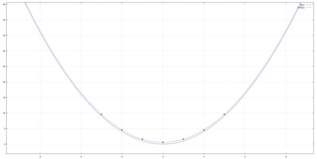
The red circles here are the points given to fit. The original function is $$ f(x) = x^2 + 0.5567 $$ The green curve is the best candidate after 185 steps and pink is the first step. The functions found by this technique however are not necessarily beautiful or easy to read. The first guess was $$ f_0(x) = 2.100\cdot 10^{-4} + (x)^2 $$ step 185 was $$ \begin{align}f_{185}(x) &= ((x \cdot (x + (3.28 \cdot 10^{-14} \cdot (((-0.717 \cdot (x + 89.84)) \\ & + (0.549 + ((-0.354 \cdot x) \cdot 94.98))) \cdot ((x + (x \cdot -0.059)) + \\ &(((-35.21 + x) \cdot (x + -22.28)))^2))))) + 0.556)\end{align}$$
As another example we consider $$ f(x)=sin(x^2) \cdot cos(x) + x $$ which we try to approximate with the same scheme. We pass the values of the exact function for the x-values \(x \in {-5,-4, \ldots, 5}\). In the following graph, the numbers in the function name give the generation that function is from and the function is always the best approximation of its generation. So \(f1(x)\) is the best approximation in generation 1, \(f30(x)\) in generation 30 and so on. \(f(x)\) is the plot of the exact function.
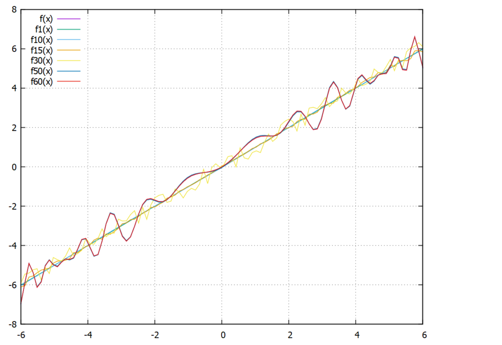
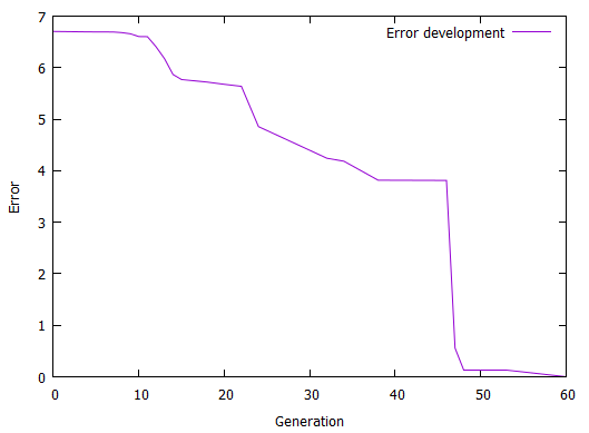
We see that the early attempts (\(f1(x)\) and \(f10(x)\) are basically straight lines somewhere near the exact solution. In generations 15 and 30 we begin to see oscillation that tries to approximate the exact behavior and 50 and 60 are so precise they cover the exact graph completely. The next plot shows how the error has evolved over time (generation):
As an example, here are some of the functions the algorithm considered. These are always the best of their generation:
| Generation | Term |
|---|---|
| 0 | \( 0.9998 x \) |
| 15 | \( x + (-0.02778 \cdot (x \cdot cos(((354.27 \cdot x^2) \cdot (((x \cdot 1.008) + x) + -3.575))))) \) |
| 46 | \( x + (-0.4849 \cdot sin((( -2.03379 \cdot x) \cdot x)))\) |
| 60 | \((((-0.3096 \cdot -7.496) \cdot -1.009 \cdot 10^{-6}) + x) + (sin((x \cdot x)) \cdot cos(x)) \) |