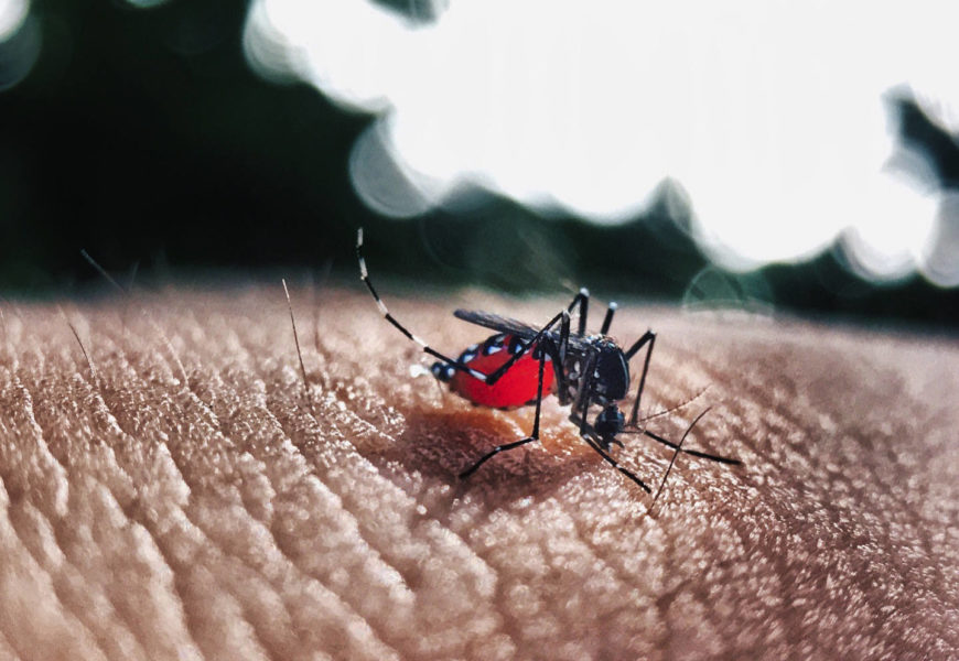
In my first blog post, I want to revisit some work I did 2 years ago for an exercise class that I helped tutor in 2017. Recent reports about Dengue Fever in Yemen and the Coronavirus in China and the US reminded me of it and that’s why I share it with you today. If you want you can read this article to learn something about the SIR-method, or alternatively, if you want to put your programming skills to the test, you can use it as an exercise for the implementation of a fairly basic numerical scheme. Either way, I am looking forward to your feedback.
To show you what we are going for: This video shows a measles outbreak spreading through my hometown of Karlsruhe. We assume a low vaccination rate and a fairly basic traffic model. If you have Matlab installed on your computer, you can simply download the .zip at the end of this post, run the solution file in it and produce the same video.
The setting
Yemen has seen many horrors in the last decades. Engulfed by a civil war that has lasted for nearly one decade, the country has seen revolts, violence, famine, and war. There is, however, another horror the people of Yemen have been forced to endure in their state of isolation from foreign aid: disease. There are reports of cholera outbreaks and, more recently, of a dengue fever outbreak.
It is hard to comprehend the horror of war or the suffering famine induces. However, I want to use something I did in an exercise class some years ago to visualize the spread of diseases such as Dengue Fever.
There is a methodology for the modeling of infectious diseases like these called the SIR model. It splits a given population into the following groups:
- \(S\) for susceptible: The group of people who can be infected with the disease in the future. This is the non-vaccinated part of the population.
- \(I\) for infected: These people are the ones, that currently both have and spread the disease.
- \(R\) for recovered: This group of people has passed through the infected stage and has “recovered”. For a potentially fatal disease, this can also mean that members of this group can have passed away. The fatality rate of a disease is typically defined as the fraction of the group of recovered people that die from the disease.
The model then defines probabilities for patients to pass from \(S\) to \(I\) (infection risk) and from \(I\) to \(R\) (recovery rate). Mathematicians determined that for example for a population of Germany it would not be enough to split the population into three groups that affect each other. That would mean, that an infected patient in Berlin could infect a susceptible person in Bavaria. A model that takes position, movement, and interaction into account, was required. Such a model was described in the publication “SIR-network model and its application to Dengue Fever” by Lucas Stolerman, Daniel Coombs and Stefanella Boatto.
This model requires the following additional data for a set of regions:
- How many people live in the region and
- How many people travel to which other regions (for each of the regions). This describes how many people from a certain region travel to any given other region often enough to infect somebody.
The model then defines each of the groups \(S\), \(R\) and \(I\) for each of the regions and models the transitions for each region. Details about this scheme can be found in the publication mentioned above.
If you are interested in the effect vaccination has on the spread of a disease (for example the recent measles outbreaks in areas of weak vaccination) or how the flew spreads through your city, the following task might be interesting for you. It requires basic knowledge in numerics and partial differential equations.
The Task:
In the following, we will examine the spread of a disease through a city. The implementation will be done in Matlab for which help will be provided. The basis for this work is the publication mentioned above.
Introduction:
$SIR$-models (Susceptible-Infected-Recovered) are a tool in the field of mathematical epidemiology to model the spread of diseases. As mentioned in the name of the method, the population is divided into three groups \(S\), \(I\) and \(R\). Aspects of population models like newborns and mortality are ignored since they are relevant only on larger timescales. Since the people who die from the disease are also counted in the \(R\)-group, the total population \(S+I+R\) is therefore constant across time – we only ask how many people are in which group at any given time. As mentioned above there are two possible movements between the groups:
- Infection is the event when a person moves from the \(S\) group to the \(I\) group. This is described by the infection rate \(\beta\).
- Recovery or death which describes people moving from \(I\) to \(R\) and is modeled by $\gamma$.
In this model, a person in the group \(R\) cannot be infected again and will therefore always stay in \(R\).
We can now derive the following basic equations:
$$ \frac{\mathrm{d} S}{\mathrm{d} \,t} (t) = – \beta S(t) \frac{I(t)}{N} , $$
$$ \frac{\mathrm{d} I}{\mathrm{d} \,t} (t) = \beta \, S(t) \frac{I(t)}{N} – \gamma I(t) ,$$
$$ \frac{\mathrm{d} R}{\mathrm{d} \,t} (t) = \gamma \, I(t), $$
with \(S,I,R \in \mathcal{C}^1([0,T], \mathbb{R}_+)\), \(\beta, \gamma, T \in \mathbb{R}_+\).
Info: In case you are not used to reading partial differential equations, the three equations above read as follows:
- The rate at which \(S\) changes over time (\(\frac{\mathrm{d} S}{\mathrm{d} \,t} (t)\)) is defined as (the number of people currently susceptible (\(S\))) times (the probability of an infected person infecting someone (\(\beta\))) times (the number of infected people (\(I\))) divided by (the total number of people(\(N\))). The minus is there because if a lot of people get infected, the number of susceptible people decreases. So:
– if there are more infected people the rate increases (makes sense).
– If the rate is more infectious, more people are infected (makes sense).
– If the percentage of people infected (\(\frac{I}{N}\)) is high, more people get infected (makes sense). - The rate at which the number of infected people increases over time is the same term only with another sign because as \(S\) gets smaller \(I\) grows. The additional term \(\gamma I(T)\) is the rate of recovery times the number of infected people, which equals the number of people who recover. So the second term describes people moving from \(I\) to \(R\). Since they leave \(I\), there is again a minus sign.
- The third equation simply states: Recovery rate times number of infected people is how many new, recovered people we get.
We will also use \(N := S(t) + I(t) + R(t) = \text{const} \). We then extend the three groups into a set of groups to model geographic factors such as proximity.
The the given city of \(M\) districts we build a SIR-network for every district and introduce coupling terms for the districts. Let \(N, S, I, R \in \mathcal{C}^1([0,T], \mathbb{R}_+)^M\) and a given matrix \(\Phi \in [0,1]^{M \times M}\) where \(\Phi_{i j}\) is the fraction of people from district \(i\) who travel to \(j\) regularly for work. That yields \(\sum_{j=1}^{M} \Phi_{i j} = 1 \forall i \in {1 , \ldots, M}\). We define the vector \(N^{\text{tot}}\in \mathbb{R}^M\) consisting of the components
$$ N_i^{\text{tot}} = \sum_{m=1}^M \Phi_{m i} N_m, $$
Which describes how many people work in district \(i\). In the publication mentioned above, the authors introduce the following equations for a SIR-network:
$$ \frac{\mathrm{d} S_i }{\mathrm{d} t} (t) = \, -\sum_{j=1}^{M}\sum_{k=1}^{M} \beta \, \Phi_{i j} S_i(t) \, \frac{\Phi_{k j} I_k(t)}{N^{tot}_j}, $$
$$ \frac{\mathrm{d} I_i }{\mathrm{d} t} (t) = \, \sum_{j=1}^{M}\sum_{k=1}^{M} \beta \, \Phi_{i j} S_i(t) \, \frac{\Phi_{k j} I_k(t)}{N^{tot}_j} – \gamma I_i(t), $$
$$ \frac{\mathrm{d} R_i }{\mathrm{d} t} (t) = \, \gamma I_i(t). $$
It is important to understand the exact meaning of these equations (this is where your basic knowledge of partial differential equations comes in handy). Focus especially on \(\Phi_{i j} S_i(t)\) and \(\Phi_{k j} I_k(t)\).
Application:
We intend to apply this model to the city Karlsruhe. The city is split into 27 districts and I will provide you with a function in Matlab to draw a map of the city with each district colored to visualize how many people there are infected. This function requires a vector consisting of 27 components describing the fraction of the population currently in the group I in that district.
We will also provide a function that generates the matrix \(\Phi\). Inside a new folder create a script file and copy the provided .m-files into it. To solve this problem we first set the timestep \(\Delta t = 1\) and a total simulation time \(T = 100\). In each timestep, compute the terms \(\frac{\mathrm{d} S_i }{\mathrm{d} t} (t), \frac{\mathrm{d} I_i }{\mathrm{d} t} (t)\) and \(\frac{\mathrm{d} R_i }{\mathrm{d} t} (t)\) and perform the update \(X(t+\Delta t) = X(t) + \triangle t \frac{\mathrm{d} X }{\mathrm{d} t} (t)\) for \(X \in {S,I,R}\).
Diseases have a biological property called the basic reproduction number (more details can be found on Wikipedia for example) which is defined as \(R_0 := \frac{\beta}{\gamma}\). First, we want to model the common cold. To model the properties of this particular disease we set \(\beta = 0.5\) and \(\gamma = 0.25\). We also set \(\triangle t = 1\) [days]. Create graphs of the number of infections for single districts and also plot \(N(t)\) over time. What do you see?
Next, we will model different diseases. Setting \(\beta = 3.75\) and \(\gamma = 0.25\) models a measles outbreak for example (for a vaccination rate of 0%). What do you notice? How can these problems be solved?
Additional task:
Possible extensions of the task.
- Find parameter values \(R_0\) at https://en.wikipedia.org/wiki/Basic_reproduction_number
- You can also specify a custom infection rate \(\beta_m\) for individual districts. This can be used to model rates vaccination coverage or travel patterns of workers.
- You can vary the initial Infection \(I(0)\) and see if an outbreak still occurs.
- \(\beta\) or \(\beta_m\) can be chosen to be dependent on the simulation time. This could be used to model a change in behaviors based on the beginning of the spread of disease.
- \(\Phi\) is an approximation of realistic couplings of the districts to each other. Can you come up with a good one?
I will append a zipped folder containing a .m-file you can start with (task.m) and an example of how the solution could look (solution.m). Have fun!
Click here to download the zip file!


